4 lasertrapr: a computational tool for automating the analysis of laser trap data
4.1 Introduction
The laser trap (or optical tweezers) has been revolutionary to the field of single molecule biophysics. Originally developed by Arthur Ashkin of Bell Laboratories (Ashkin 1986) the laser trap was eventually adopted by biologists to study the interactions of single molecular motors (e.g. myosin, kinesin, dynein) with their molecular tracks (e.g. actin, microtubules) by use of a three-bead assay (Finer, Simmons, and Spudich 1994; Kojima et al. 1997). These experiments permit researchers the ability to observe the interaction of two proteins within a millisecond-time and nanometer-spatial resolution providing unprecedented insight into the molecular machinery underlying a wide variety of biological functions including muscle contraction, intracellular cargo transport, and cell-division. Such experiments need to be performed with a low trap stiffness (0.02-0.04 pN/nm) as to not hinder the function or harm the integrity of the experimental proteins or setup. Since the position of a trapped bead is largely dominated by Brownian forces, a bead stuck in a trap with low stiffness has a large variance in its displacement signal as trap stiffness (\(\alpha\)trap) is inversely proportional to the variance (\(\sigma\)2) of the displacement signal (via the Equipartition Theorem) Svoboda and Block (1994).
\[ \alpha_{trap} = \frac{ k_B T_k } { \sigma^2 } \]
where kB is the Boltzmann constant and Tk the temperature in Kelvin. The high variance of the baseline displacement signal combined with the dampening effects of viscous drag forces masks the underlying mechanics of the two proteins interacting and cycling through a mechanochemical scheme that is common amongst biological motors used in these assays which makes the analytical task of identifying these events of interests quite challenging.
The variance of the displacement signal is a crucially important feature of single molecule laser trap data as the variance can be exploited to determine when protein interactions do occur. Since the biological motors used in these experiments are stiffer than the trapping laser, the interaction of the proteins can be characterized by a decrease in signal variance of the time series (position over time) signal, via Eq 1, which is also often accompanied by a displacement from the mean baseline position as in the case of a biological motor, like myosin, attaching to an actin filament and performing a powerstroke. In some cases, the signal-to-noise ratio of the baseline and event populations variance can exceed 2:1 which makes these interaction events readily discernible “by-eye”. However, while simple and easy, the analysis of data “by-eye” has been criticized in the past as this method was suggested to introduce subjectivity via user bias as evidenced by early inaccurate estimations of myosin’s displacement size (Finer, Simmons, and Spudich 1994; J. E. Molloy et al. 1995b). This exemplifies the fact that while the laser trap is a powerful and advanced scientific instrument, the reliability and accuracy of the information that can be extracted from the resulting data is limited by the validity of the techniques and programs used to analyze the data. While there are numerous techniques that can be used to identify binding events, a common theme between them is that most require advanced computer programming knowledge to implement. This is then compounded with a need to then automate those scripts by a preferential creation of user-friendly graphical user interfaces (GUIs). For most, the advanced computer skills required to build sophisticated analysis programs with GUIs are taught in classes that are not degree requirements for graduate students or researchers seeking degrees in many biology-related fields. This presents a technological barrier that hinders progress in understanding and interpretation of data for new students and researchers, and an additional monetary cost barrier is added to a laboratory if the creation of custom program must be outsourced. And, even in these situations then a research group is left with an custom and un-supported “black-box” program.
Unfortunately, there are currently no completely open-source projects whose primary aim is to automate the workflow of analyzing laser trap data (calibrations, processing, event identification, ensemble average, and summarizing statistics) written with an open-sourced programming language. Although it should be noted there have been recent publications of programs aimed at single molecule event identification, most notably the MATLAB based SPASM (Software for Precise Analysis of Single Molecules, Blackwell et al. (2021)). However, while SPASM itself is an open-source program, the underlying MATLAB language is proprietary/closed source language and has a steep financial barrier (currently a standard MATLAB license has an annual fee of $860 per their website at the time of writing). Here, we present {lasertrapr}, and open-source program for automating the analysis of laser trap data written in R, a free and open-source programming language (hence lasertrapr = laser trap + R; also note that it is common in the R-community to denote R-packages with {}). The tool has an easy-to-use GUI provided by the R-Shiny web-framework package. One of the main benefits of having a tool built with R/Shiny (R Core Team 2022; Chang et al. 2021) is that there is high portability of the app across different operating systems as it can be installed on Windows, MacOS, and Linux systems. Additionally, we do not view our application as a replacement or competitor to a program such as SPASM, but as an additional tool made available to the biophysics community that has some similar features (single molecule event identification and ensemble averaging) but for distinct data types (SPASM’s main event identification is built for 2 QPD systems using co-variance of bead position whereas our is for a 1 QPD system). Furthermore, {lasertrapr} fully embodies the notion of a free and open-source project whose main goal is automation and reproducibility of the entire workflow of analyzing laser trap data which includes folder/file creation and organization, signal calibrations, data cleaning and preparation, event identification of both single molecule and mini-ensemble data, ensemble averaging, generation of complete project summary statistics, and creation of publication quality figures. Lastly, the co-existence of multiple programs will only benefit the biophysics community by enabling researchers the ability to contribute to and use an analysis program best suited for their interests and experimental setups.
4.2 Results & Discussion
The following Results & Discussion serves as both a validation of the app and provides example use cases of what can be accomplished within the app. The paper presented in Chapter 5 was analyzed completely with this app so the present chapter’s aim is to provide evidence that the app provides a reproducible, precise, and accurate analysis tool. While reading this section if you decide that you really like the app and would like to try it yourself, there is a user-guide and complete documentation on how to install and use the app available on the app’s website https://lasertrapr.app/ including example videos. The documentation is also included in section 4.3. Additionally, the project can be found on Github at https://github.com/brentscott93/lasertrapr.
4.2.1 Single Molecule Analysis Validation: Simple
One of the main features of the app pertains to the analysis of single molecule laser trap data. Here, we will validate the single molecule analyzer that is based on a combination Hidden-Markov Model + Changepoint analysis. The full details of the analysis are provided in section 4.2.7 which walks through the actual single molecule analysis line-by-line. These tests will verify that the app can identify actomyosin binding events using simulated data which provide ideal and known conditions. In thie first simulation, every event has a 5nm displacement and 100ms attachment time. The single baseline-event-baseline data set is shown in Figure 4.1.
A simulated laser trap event. The event has 200ms of baseline preceeding a 5nm displacement that lasts for 100ms. Another 200ms of baseline data is appended after the displacement. This exact sequence was replicated and concatenated together 200 times which yields a data trace with 200 simulated binding events that are spaced 400ms a part. The exact simulated measurements are: 5nm displacement, 100ms attachment times, and 400ms time between events.
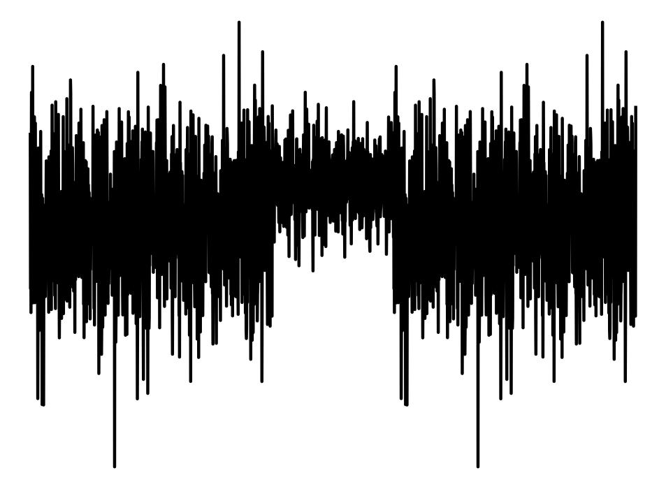
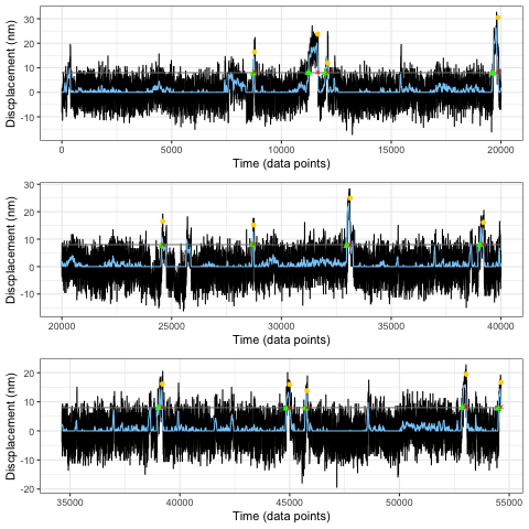
The 200 event simulation was analyzed to test the number of events the analysis could detect out of the original 200 created. One of the features of the app is that after the analysis it takes the original raw/simulated trapping data and “overlays” the analysis results on-top of the original data so the user can compare/check how the analyzer is performing. A screenshot of the results of the analysis provided by the app is shown in Figure 4.2. If you were using the app the figure displayed in Figure 4.2 would be an interactive graph that would allow you as a user interactive abilities to pan across the data and the analysis. This feature allows the user to become more familiar with their data and the app’s output.
Screenshot of the output from the single molecule analysis produced by lasertrapr. Black lines is the original trap trace, the green line signifies the results of the hidden markov model performed on the running window transormation, and the yellow highlights is the final results after changepoint is applied.
The output of app’s estimation of the displacement and attachment time for the 200 event simulation is shown in Table 4.1. The results show that the analysis correctly identifies and measures single molecule binding events. The app estimated a 5.1nm displacement and 99.8ms attachment time which accurately represents the known simulated values of 5nm and 100ms. Indeed, the 400ms time between events is also the same as the simulation input.
| displacement_avg | time_on_avg | time_off_avg |
|---|---|---|
| 5.109922 | 99.8 | 400.0251 |
4.2.2 Single Molecule Analysis Validation: Adding Complexity
4.2.2.1 Simulating displacement distributions
Adding complexity to the simulations creates more realistic datasets that allows for more robust testing and assurance in the precision and accuracy of the program. In the previous data example, every event had the same exact displacement and attachment time. Here we simulate displacement distributions which more accurately represents how real single molecule data would be collected. Since each displacement in the trap is the summation of the displacement caused by myosin’s powerstroke and that of random brownian noise, displacement data in the single molecule laser trap have been shown to be normally distributed with a mean displacement equivalent to myosin’s powerstroke size and standard deviation that is dependent on the trap stiffness (J. E. Molloy et al. (1995b)).
Four datasets were simulated whose event population had displacements generated from four distinct Gaussian distributions whose mean values were 0, 5, 10, and 15nm, respectively. Being able to detect 0nm displacement events was an important test to conduct considering the possibility for the “slow mouse” S217A mutation to actually have a small or even no displacement as described in Chapter 1 within Aim 2. The data was analyzed with the single molecule analyzer within the app and summarized in Figure 4.3. The app’s estimated average displacement was modeled against the actual average displacement of the Gaussian distributions that generated the data and fit with a linear regression. The coefficient of determination (R2) is 0.99 indicating that the analysis is able to accurately predict average displacements across a wide range of distances. Additionally, out of a total of 4000 simulated events the app identified 3997 which is a 99.925% detection rate for these simulations.
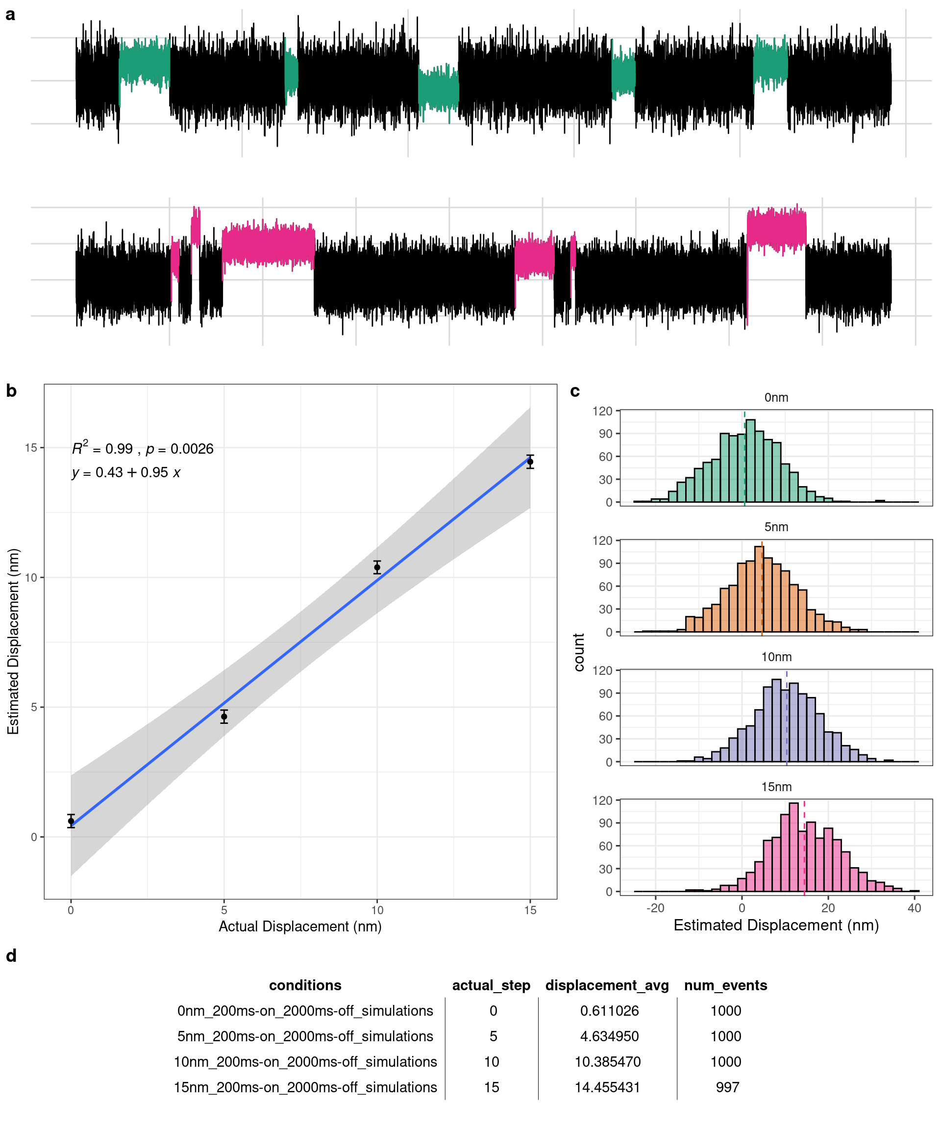
Figure 4.1: Four simulations were performed with average dispalcements of 0, 5, 10, and 15nm. a) Simulated data traces. Top trace has 0nm average displacement. Bottom has a 15nm average displacement. b) Linear regression of the actual displacement (x-axis) versus the analysis estimated displacement size (y-axis) demonstrating a near perfect correlation. c) Full gaussian distributions of the analyzer’s estimated displacement for each of the 4 simulations.
4.2.2.2 Simulating attachment time distributions
In similar fashion to the displacement distributions, the attachment lifetimes for each myosin binding event is not the exact same for each interaction. The total event population for myosin’s attachment time is exponentially distributed, so we simulated additional data where we defined exponential distributions to generate total attachment times from for each event. Truncated exponential distributions were used in order to more easily generate data that would be confined to the needs of the simulations. For example, in the case of an exponential distribution and as the the PDF suggests, the smallest numbers are the most probable to generate upon random sampling. However, when simulating data we are confined to defining time in terms of datapoints per the sampling frequency. To avoid randomly generating infinitely small ADP-release/ATP-binding rates, which define the total attachment lifetimes, the exponentials are truncated at a minimum of 1 or more milliseconds. Additionally, a truncation of minimum attachment-times also increases the assurance that if we generate 100 events the simulator will actually simulate 100 observable and detectable events. For these sets of simulations, the rates supplied to the exponential distributions represent the average attachment lifetime of the population since for a given exponential distribution the arithmetic mean (expected value) is equivalent to the reciprocal of the decay rate \[ E[x] = 1/\lambda \]. Drawing a random value from each distribution yields the length of time that the attachment time should be to for a given event. Each distribution shown below reflect 10,0000 random draws from a respective distribution whose rate are 20, 10, 5, 1 with lower bounds of 0.02, 0.02, 0.02, 0.02 and upper bounds of 0.3, 1.856, 1.856, 3. As shown in Figure 4.4, decreasing the rate increases increases the time values that can be generated which results in longer attachment times. Furthermore, panel C represents exponential distribution with the same rates used except panel C is not-truncated. The distributions in panel C further display the use-case for truncating the data to make more economical (i.e. smaller file sizes) as it is an attempt to to avoid excruciatingly long attachment/detachment times when the rate constant is 1. For these simulations, the ATP binding rate was set to take 1ms (5 data points) on average, so its attachment time contributions can largely be ignored which made the comparisons easier. This would be analogous to conducting experiments at a very high ATP concentration (>1mM). Essentially as soon as ADP is released a new ATP is readily nearby and instantaneously can bind to myosin’s active site causing a detachment.
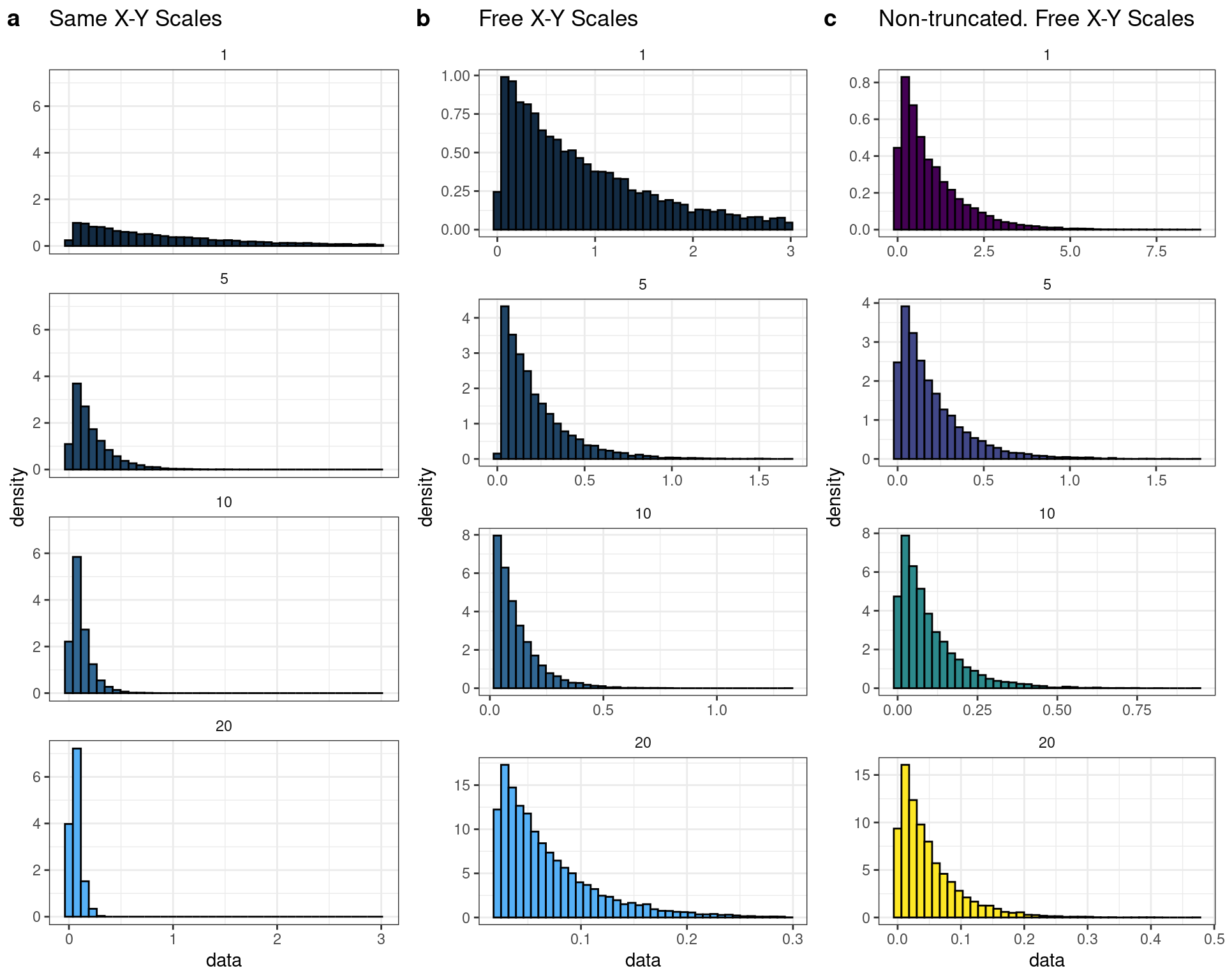
Figure 4.2: Simulated truncated (a & b) exponential distributions that are representative to the ones used to generate the simualted data
The data was analyzed with the single molecule analyzer where the attachment lifetimes were estimated by the app and then compared to the true values set in the simulations. Since truncated exponential distributions were used, the average attachment time is not as simple as taking the reciprocal of the decay rate. To get an estimate of the possible true rate/attachment times generated from the truncated distributions, 10 rounds of 10,000 random draws from the truncated distributions were generated. For each 1 set that contained 10,000 random draws the average was recorded (0.068759, 0.0693254, 0.0696117, 0.068123, 0.0689889, 0.0690398, 0.0698608, 0.0693016, 0.0689494, 0.0684859) and then those averages were averaged together to be compared against the mean attachment time as estimated from the app. The estimated attachment lifetimes were modeled against the known/true values, and fit with a linear regression. The coefficient of determination (R2) is 1 indicating that the analysis can accurately estimate attachment lifetimes for a wide variety of time periods indicating that the app/analysis should be able to be applied to a wide variety of myosin/molecular motors with differing ADP release rates and even under experiments at higher ATP conditions which decreases the attachment times.
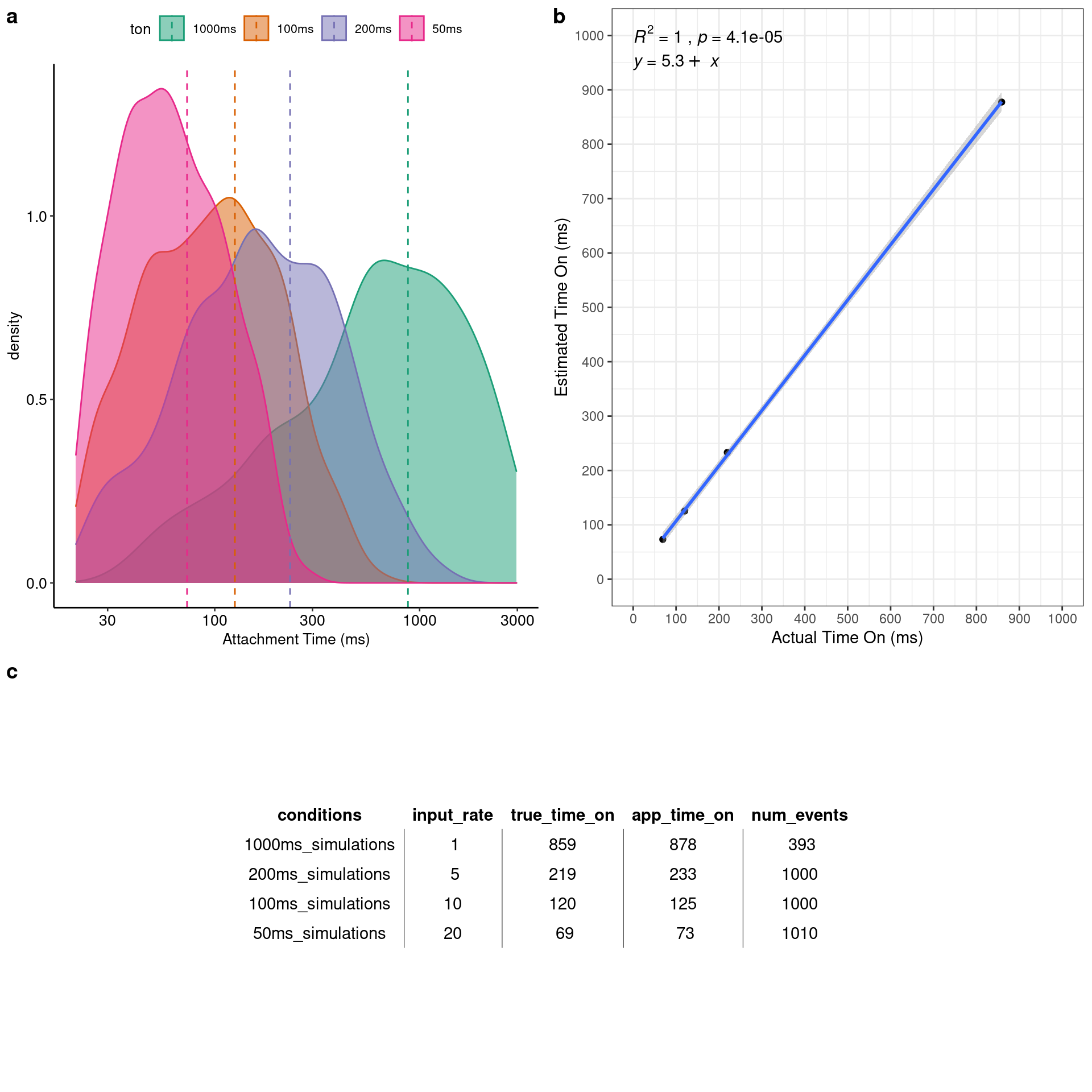
Figure 4.3: Four simulations were performed with average attachment lifetimes of 50
4.2.2.3 Short Events
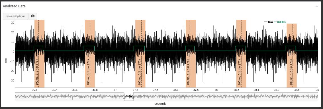
To further test the single molecule analyzer and test the limitations of reliable event detection a dataset was simulated with very short attachment times (~20ms average). The window width of the HM-Model was decreased to 100 datapoints making the event more readily detectable. Figure 4.6 shows the identified event in this short event simulation The data was simulated, analyzed and even Figure 4.5 was generated from within the app with the built-in “screenshot” tool which makes saving snippets of analyzed traces easy and provides color coding of identified events free of charge.
Figure 4.4: Simulated data trace with very short events. Measured attachment times for the 3 ID’d events in the trace are 18, 15, and 32ms. Plot is interactive online. Grid lines represent 1s and 2nm intervals.
4.2.3 Accuracy of determining beginning and end of events
The single molecule analyzer built using the HM-Model/Changepoint analysis will estimate the start or end of event by returning the exact datapoint in the original raw trace that the analyzer chooses as the most probable start/end for each event. We can compare the app’s estimation of the start/stop of each event with the true start/stop datapoint at which the event begins/ends by using a simulated data trace as the information about the exact datapoint that the event starts/ends is truly known by the simulation. Figure 4.6 shows the average/median number of datapoints that the estimation differs from the known values and the estimated values. Each histogram is inset with a cumulative distribution. In Panel A, the cumulative distribution for the start of the events can be interpreted as ~75% events are being chosen within 2ms (10 datapoints) of the true starting datapoint. The table in panel “C” of Figure 4.7 shows the values of the misalignment calculations which were calculated by subtracting the datapoint index of the true start/end of each event (a known value from the simulations) from the app’s estimation of the start/end of the event (i.e. startapp - starttrue). If the value of the misalignment is negative this would indicate that the app’s estimation of the start/end datapoint index tended to be a smaller number than the true value. This would mean that the app tends to start the event early and that the app is estimating the event to start before the event known start occurs. Looking at the comparison of the event start, the distribution appears to be more exponentially distributed than normal so the median value may have a more appropriate value of to describe the data with. The median has a value of -3, which indicates that 50% of the events are misaligned within the range of -3 datapoints to the maximum misalignment +8 At 5000Hz sampling frequency this is -600 microseconds to 1.6 milliseconds. Comparison of the end of event misalignment calculations, the median value is -2 datapoints, indicating that 50% of the events are misaligned between the minimum value of -8 datapoints and the median value of -2 datapoints. Converting into the time domain with a 5000 Hz sampling frequency these misalignment calculation indicate the app is terminating the events early by -1.8 milliseconds to -400 microseconds. The few larger misalignment values where the app estimates the events to end after the true stop seem to be skewing the average to a positive value, but indeed for the majority of events, the app is estimating the end of each event to be slightly before the true end as evidenced by the median value and the cumulative distributions in panel “C” of Figure 4.6.
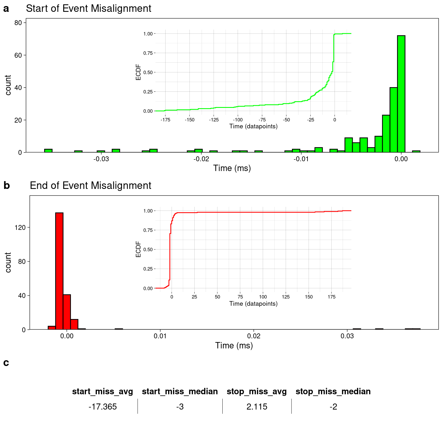
Figure 4.5: Analysis of the misalignment in the true start/end of an event and the analysis estimated start/end of an event. a) About 75% of the start of events are picked within several datapoints. b) The ends of events are mostly picked with a couple data point error. c) A table showing the average or median number of datapoints that the analysis missed the start or end of an event by.
4.2.4 Ensemble Averaging
Conceptually this process is simple, as the final step is just a mathematical average of data points. However, the process of wrangling your data to get to the final averaging step is challenging. Ensemble averaging in general is discussed in the literature review in Chapter 2, and here we will stick to the discussion of ensemble averaging in regards to the app and how it implements the technique.
The main question addressed in Chapter 5 using the “slow mouse” S217A mutation that slows Pi-release was a major motivating factor to start building single molecule event identification programs that would then permit the ability to perform ensemble averaging since prior to the start of the project we were unsure what the effects of the mutation would be, or how the severe the effects would manifest. First analysis attempts for the data was made using the Mean-Variance analysis as described in Chapter 2. However, MV would only be able to estimate a displacement distribution in attempts to see if the mutation would alter myosin’s overall displacement. This is important to note because there could be no change in the total displacement, but still the transition rate could be changed between the unbound-to-bound populations. This question was un-testable with MV since it provides a single global displacement estimate for a raw trace, which highlighted the importance of needing the ability to ensemble average the data.
4.2.4.1 First attempts
We performed ensemble averaging for Gunther et al. (2020) which was a study prior to Scott-Marang 2021 where in a collaborated effort with the Yengo & Thomas Lab we performed a wide variety of biophysical characterization of the “slow mouse” S217A mutant. The ensemble averaging for this was slightly different from previous published ensemble averages, in part because we were wanting to focus/address one specific question - does S217A slow the unbound-to-bound transition? Some major differences in ensemble averaging technique that deviated from prior work was that only the first 60ms of all each event were included, only positive displacement events were included, and we only looked at the forwards ensembles. Additionally, ensembles were fit with a single exponential that started from the origin (0,0). Figure 4.8 shows the ensembles from Gunther et al. (2020) the following is part of the methods providing further details:
“The ensemble averaged events are 60 ms long and only include events that had positive displacements. Events meeting the inclusion criteria had the back 30% of their lengths removed in preparation for event alignment. The changepoint analysis provided a new relative time index for the start of each event, and as a result the events could universally be reindexed with the same relative time scale. The first data point in each event was indexed as dp0, and thus each event was indexed as {dp0, dp1,. . ., dpn}, where dpn represents either the 300th data point (dp299) in the event (corresponding to the first 60 ms of a longer event) or the last data point of a shorter event (dp299). For short events less than 60 ms in which dpn <= dp299, the average displacement of the event was used to extend the event to length dp299. Events were then aligned horizontally at dp0, and all matching dpx values were averaged together to create the final ensemble. The average ensembles were then fit with a negative mono-exponential equation using the {drc} and {aomisc} R packages to provide estimates of the rate of the working stroke and plot with the {ggplot2} and {cowplot} R packages. Additional programming tools used for building the analysis programs include the {gtools}, {pracma}, and {tidyverse} packages.”
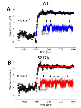
Ensemble averages created for Gunther 2020. Blue is WT mysoin. Red is the S217A mutation. All data collected at pH 7.0 and 0mM-Pi. Raw traces are inset and ensembles are fit a with single exponential.
The major conclusion from the ensembles averages in Gunther et al. (2020) was that the mutation did not have a slowed transition from unbound-to-bound compared to the WT (629 vs 867 s-1) at 0mM-Pi concentration. If anything the mutation was slightly faster, which in hindsight was due to the fact that the exponential was fit to the initial transition which included some additional data after the completion of the powerstroke. S217A was shown to have a 2x fold faster ADP-release rate in Gunther et al. (2020) from solution kinetic studies, which coincidentally explains the faster attachments times we saw in this paper for the mutation. This faster ADP-release rate would also manifest in the hitch occurring sooner as compared to the WT. In the case of these forwards ensemble averages, the exponential rate most likely reflect the rate of the initial transition plus some of the rate at which the hitch occurs. The S217A would have a higher percentage of events that would have been able to complete their hitch compared to the WT within the first 60ms. This is reflected in the slightly higher rate of the fit, but this would have no bearings/effects in regards to the validity of the analysis in answering the primary question.
4.2.5 Testing the Ensemble Averager
As described and shown in previous sections, the {lasertrapr} app has an analyzer for identifying events in single molecule laser trapping data. This analyzer determines the exact data point where an actomyosin binding event begins and the exact data point where the binding event terminates. With this information we can “temporally synchronize” the events and average them together to create ensembles that represent the average response of the binding interactions. A simple example of the process of the ensemble alignment procedure can simply explained with two theoretical events.
Say we have two events that were both exactly 200ms, one event takes place from datapoints 5000-5999 and the other from datapoints 20,000-20,999. These datapoint indices would be returned by the analyzer as the respective beginning and ends of the events. They are both 1000 data points long making them 200ms long (assuming a sampling frequency of 5000 Hz). To average these events together, we need to “temporally synchronize” the events. In the laser trap, the collected data we obtain is a time-series (the position of the bead is recorded over time) and the events occur at differing points in time as in the example (datapoint 5000 vs datapoint 20,000). Knowing the datapoint indices of where each event’s respective start occurs in time, datapoint 5000 for event 1 and datapoint 20,000 for event 2, the events can be subset out of the original raw trace, re-scaled, and placed on similar relative time scale. Meaning the start of event 1, datapoint 5000, becomes datapoint 0 and the last datapoint of event 1, datapoint 5999, becomes datapoint 999. We still have a 200ms long event which contain the same y-axis position values, just the x-axis values changed relative to the start of the event. This same procedure is performed with the second event. Datapoint 20,0000 becomes datapoint 0. Datapoint 20,999 becomes datapoint 999. Now we have 2 events with the same relative time scale. Now we can average the y-value associated with time 0 from event 1 with the y-value associated with time 0 from event 2 together, etc. This will create a new event that represents the average of the two. This same procudure can then be performed with how every many events are occurring in the datasets for each condition.
What makes this is a little trickier than the above example is that every event is not the same length in time. While the above example provided a discussion on the average of two events of 1000 datapoints together, how could two events be averaged if one event was 1 second long and other was 200ms? During the alignment procedure the events need to be both 1) temporally synchronized starting at time 0, and 2) extended to the same length. Now in the case of 2 events that are 200ms and 1 second long, the 200ms event will be extended by 800ms. This can be accomplished by taking the average of the last few milliseconds of data within the event (datapoints 900-999) and obtain the average position value which can then be used to “extend” the event to 1 second long. Extending an event is adding/repeating data to the event to make it longer in time. So if the average y-value of the last 2 milliseconds of the forward ensemble of event 2 is 6.7nm. Then that value (6.7) is added 4000 times to the event 1 data to result in having 2 events that are both 1 second long (assuming 5000hz, 1 second is 5000 datapoint, 200ms is 1000 datapoints and so 5000-1000 = 4000 datapoints). The events can then be averaged together as described previously.
{lasertrapr} has the functionality to create ensemble averages which includes auto-generated plots and a choice of a single, double, or no exponential fits to the data. In order to test the accuracy of the app in the construction of ensemble averages two distinct datasets were simulated. In one data set, every event had exactly a 4nm step size with an accompanying 2nm hitch while the other has a 7nm step with a 3nm hitch (plus brownian noise). No displacement distribution were simulated, every event was a positive 4 or 7nm. Both the ATP and ADP binding rates were 10 set at 10s-1 for the 4+2 group and 5s-1 for the 7+3 simulations. Making the ensembles in the app is a three part process. The first step is creating the ensembles, averaging/fitting, and plotting. The app allows some user selection in creating the ensembles in regards to selecting a time period to extend the events forwards/backwards.
Care needs to be taken when extending the backwards ensembles as this process can be a little tricky. The single molecule analysis classifies the transition into an even as part of the event. Since each event is a summation of myosin’s powerstroke (d1, 6nm) and hitch (d2, 2nm) then the total displacement would be 8nm (dtotal). If you took the average position of the first 1ms, the average would reflect the transition from unbound to bound, and would results in extending backwards in time with a value that would be smaller than d1 (6nm). This would cause an accidental inflation of the size of the hitch in the backwards ensemble. To properly extend the backwards ensemble you need to average the true post-powerstroke, pre-hitch displacement, The d1 state. In the app this is accomplished by “skipping” into the event before averaging the position.
Extending the forwards ensembles is more straightforward since the single molecule analyzer does not tend to classify the transition back to baseline as part of the event. The last datapoint that signifies the end of the event in the analysis tends to be at peak displacement, so the app averages the last few milliseconds prior to this datapoint to represent the d2 post-hitch displacement to extend forward in time. The one consideration to keep in mind when extending forward is to be diligent of the ATP concentration that were used in the experiments and/or the ATP affinity of the motor used. At infinitely high ATP concentrations with a motor with an infinitely high ATP affinity creating an ensemble average perhaps may not be possible. Assuming that the hitch accompanies ADP-release, the rigor state would then be infinitely short/undetectable because the motor would spend too little of time at the post-hitch d2 final displacement segment. This would most likely result in being unable to properly extend forward the events because there would no d2 datapoint to average/extend. The extension would be from the d1 displacement which would create a forward ensemble that would appear to have no hitch solely because there would be no data to properly create the ensembles with.
The resulting ensemble averages of the simulated data are shown in Figure 4.9. The analysis was able to estimate a 3.7nm step and 2.3nm hitch for the 4+2 conditions, and a 6.9nm step and 3.2nm hitch was estimated for the 7+3 conditions. Note that the estimations of the d1 and d2 values are coming from the double exponential fits to the forwards ensmebles. The unbound/bound transition is simulated as occurring instantaneously in the app’s simulator so the initial transition rate is quite fast (>500/s) which reflects what would be seen in real data which where that rate is also usually around 500/s and is dependent on the corner frequency of the instrument reflecting the average rate of a bead being damped by viscous drag forces.
Interestingly, the rates of k1 which are associated with the rate of ADP release closely match the rates that were input into the simulations. The double exponential fits to the forwards ensembles estimate a rate of 13/s where the value of 10/s was input as the rate of ADP release of the 4+2 conditions, whereas the fits estimated an ADP release rate (k1) as 6/s for the 7+3 conditions and 5/s was the rate input.
The backwards ensembles are always fit with a single exponential which also estimates the d1 and d2 values from the fit parameters along with the rate of k2 which is generally attributed to the ATP binding constant. For these simulations the ATP binding constants were set at 10/s and 5/s for the 4+2 and 7+3 conditions respectively and the single exponential fits to the backwards ensembles estimated these rates to be 7.4/s and 5.0/s.
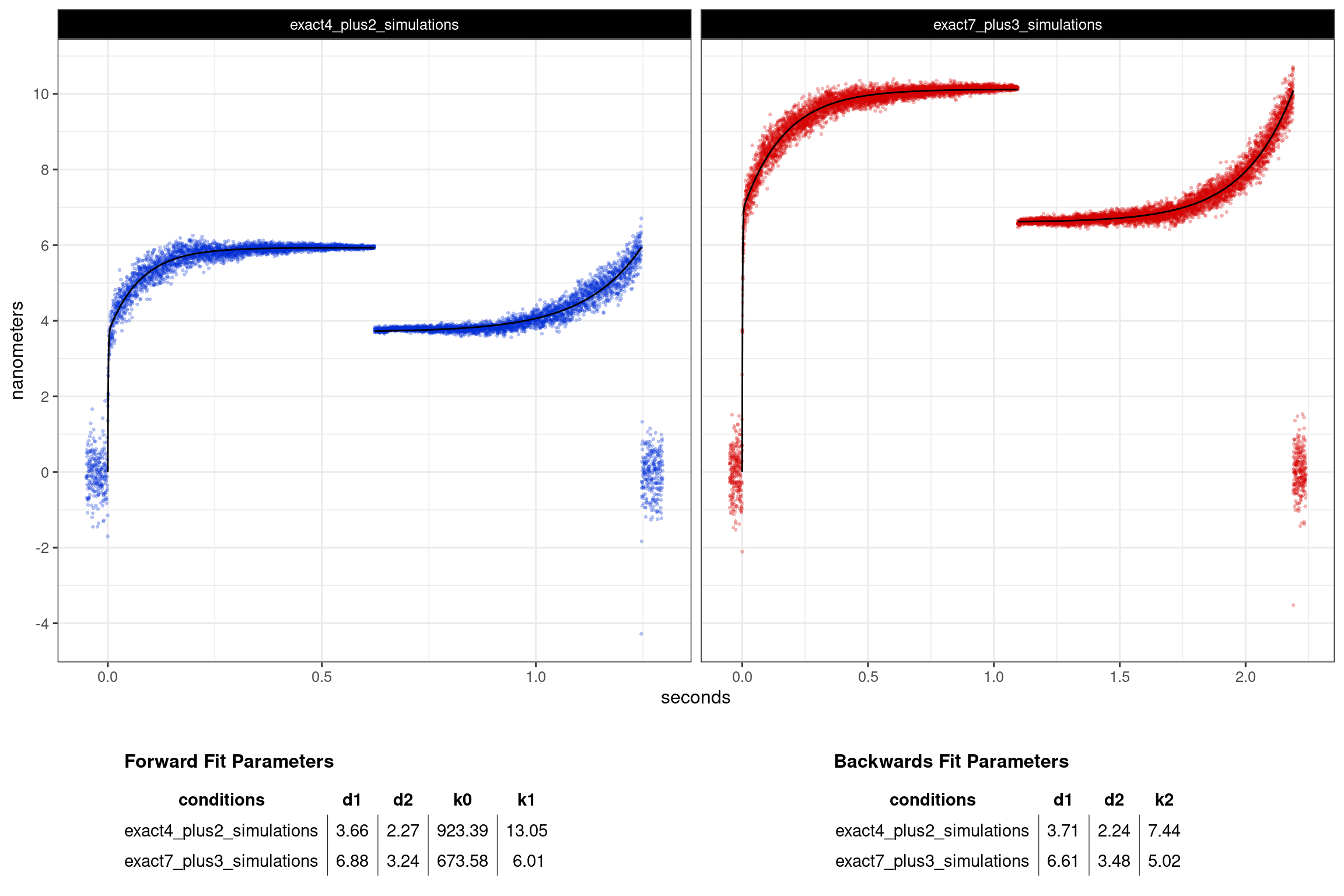
Figure 4.6: Ensmebles averages of the simulated datasets for validation. The tables show values from the fits that closely correspond to the true values.
4.2.6 Mini-Ensemble Analyzer
An additional feature of the {lasertrapr} app is the ability to analyze mini-ensemble laser trap data. The mini-ensemble assay is the exact same assay as described for these studies performed for this dissertation in Chapter 5 except with more myosin on the surface. In the mini-ensemble laser trap assay multiple myosin heads can interact/bind to a single actin filament causing rapid displacement, or “runs”. This assay displays the ability of a team of molecule motors to create larger ensemble forces when allowed to work together. The mini-ensemble analyzer in the app was a recreation of prior published work from the lab (Longyear, Walcott, and Debold (2017)). Briefly, raw data is low-pass filtered using a running mean with a window width that can be variably set by the user (typically ~10 ms, 50 data points at the sampling rate of 5kHz). Events are then identified using two criteria: 1) a user defined displacement threshold is set to the running mean to signal the start or end of an event, and 2) the event meets/exceeds a minimum defined attachment time. Attachment duration can then be calculated as the time between the start and end displacement thresholds. The time between events can be calculated as the time between the end of an event and the start of the subsequent event. Peak forces can be estimated by by identifying the maximal displacement of each record and converting the displacement into forces, by multiplying the peak displacement by the combined trap stiffnesses.
An early output plot from the mini-ensemble analyzer. The plots are now scrollable/interactive, but this serves as a fun reminder of where the app began in its infancy years prior to its creation.
This analyzer was used in Woodward et al. (2020) to compare the effects of an abiotic triposphate compound that was altering myosin’s behavior. The data analysis helped provide invaluable insight into understanding the mechanisms of the decreased force producing capabilities of myosin when it used the ATP alternative compound as substrate.
Image from Woodward et al. (2020) showcasing the mini-ensemble analyzer that is now a core feature within the app.
4.2.7 Single Molecule Event Identification (step-by-step)
This is a “step-by-step” walk through of the Hidden-Markov/Changepoint Analysis we use to analyze our single molecule laser trap data and includes everything on the journey from raw data to analyzed trace and everything on the way…buckle up. This section is a lot cooler if you are reading online and includes the R code to reproduce this by hand. You can download the data here
4.2.7.1 Raw data
Here is a raw data trace. This is unprocessed data as-is from the trap computer. The data is relative position of the bead in mV over time:
Figure 4.7: Raw trap data.
The data record is 89.1576 seconds long and has an average position of 6.2968527 mV.
4.2.7.2 Processed Data
The first step of the analysis is removing the “baseline” by centering the mean around 0. This can either be done by simply subtracting the baseline mean from every data point or by performing a piecewise linear detrend on the whole record. The latter accomplishes two things: 1) Centers mean around 0 and 2) removes any drift (i.e. wander correction). Additionally, in the {lasertrapr} app you can find the average baseline position by using a mean variance transformation of the data to select the baseline population or by selecting a quiescent period of the data where no binding events occur to calculate mean baseline position. Here we will detrend the data and convert from mV to nm using a “Step Calibration”. The step calibration is performed by moving the microscope stage a known distance, say 200 nanometers, and measuring the resulting change in the mV signal. We then can estimate the number of nanometers per mV.
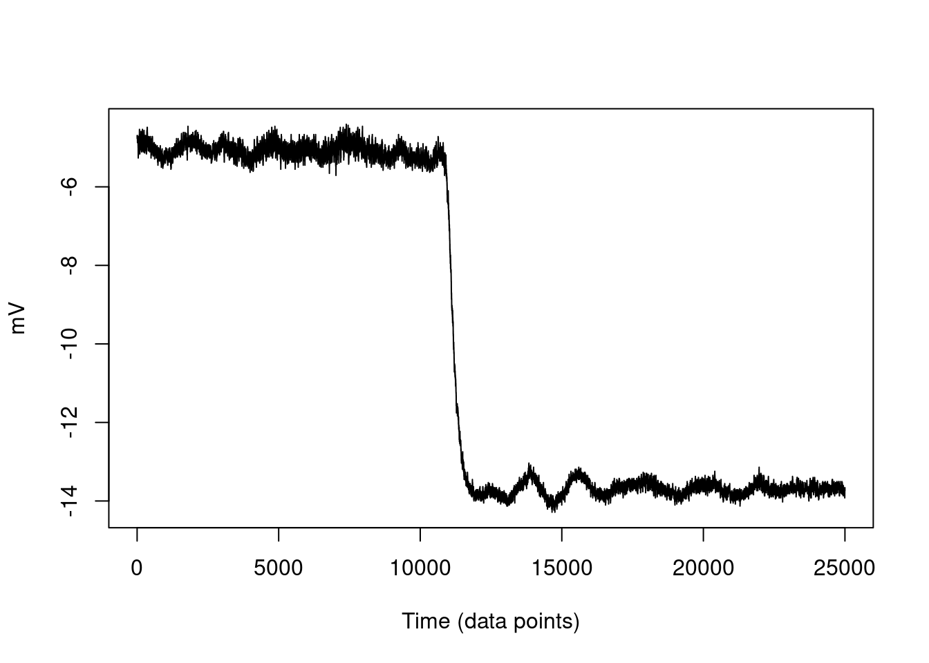
Figure 4.8: Example of a step calibration. Stage was moved 200nm
The mV-to-nm conversion calibrated around the time this data trace collecting we are analyzing know was 30 nm/mV. We can convert our raw data from mV to nm and detrend the data (or visa versa).